Playing around with TensorFlow in the browser

TLDR: I made a game of snake in which you control the snake by pointing your head. It uses your device’s camera and a pretrained TensorFlow model to estimate the direction your head is pointing in.

A week ago or so I decided to take on a hobby programming project. I wanted to make something involving machine learning that was somehow interactive, and I wanted it to run in the browser so that it could be hosted with GitHub pages to minimise worries about servers.

I knew that one of the clever things about TensorFlow is that it makes it relatively straightforward to run a trained model on various platforms, so I looked into TensorFlow.js as a way to run models in the browser.

As a first mini-project in this direction, I made a digit-classifier trained using MNIST. Here’s a demo:
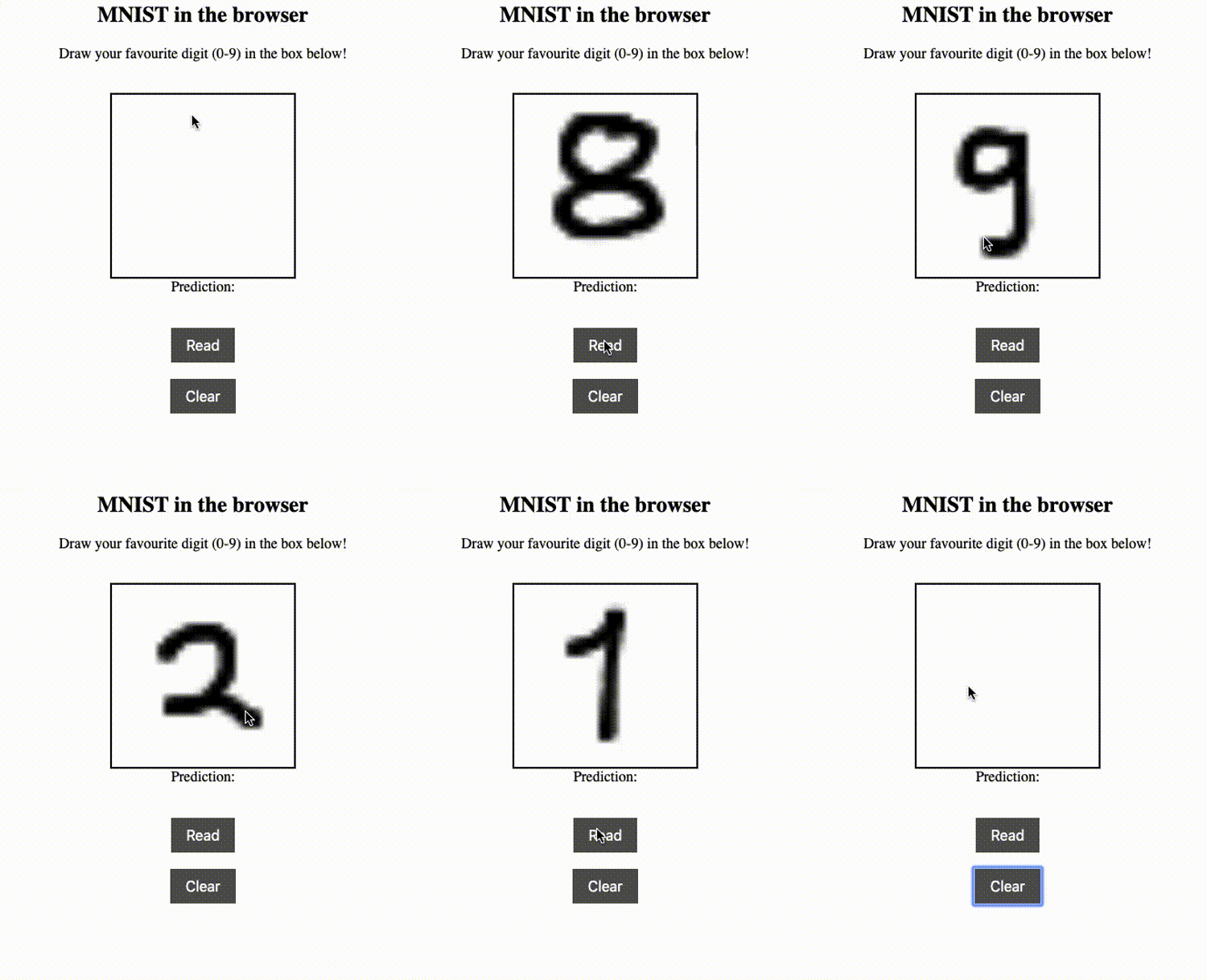
You can see the live version here, and the code on GitHub here.

Training the model was nothing new to me, but having never properly learned JavaScript, there were many things that I had to learn by debugging. Here are a few things I learned about: drawing on a canvas; converting a canvas into a grid of pixels; asynchronous functions (I still don’t understand how to properly deal with promises and “thenable” objects to be honest); disabling pull-to-refresh.

Now armed with the knowledge of how to actually run TensorFlow models in the browser, I decided to make something slightly less trivial. While looking through the TensorFlow.js examples, I saw a demo of a model that estimates the geometry of faces from 2D images. I thought this was cool and wanted to make something with it!

The simplest non-trivial thing I could think of was to use the model to estimate the direction that the user’s head was pointing in — up, down, left, right or straight ahead. I had previously made a game of snake as a warm-up JavaScript exercise and thought it would be cool to be able to play by moving your head rather than using the keyboard to control the snake. Here’s a demo:

The live version is here, and the code is on GitHub here.

I’ll briefly explain in the rest of this post how the head-direction estimation works. (The actual snake part of this is just straightforward basic JavaScript, so I won’t discuss that here.)

The face mesh model from the TensorFlow.js examples accepts an image as input and outputs estimates of the 3-dimensional locations of ~400 facial landmarks. These points form the vertices of a mesh that describes the face. For instance, there are ~10 points determining the boundaries of the upper and lower lips and each eyelid. Although the model outputs locations for all of these landmarks, we only make use of a few.

The high level idea is to model the face as a flat plane, and to estimate the normal vector of this plane. That vector points in the direction that the face is looking. To find the normal vector of any plane, you can take any two non-parallel vectors lying in the plane and take their cross product.

Here, we locate the centre of the mouth by averaging the coordinates of the lip landmarks. We also locate the left and right cheeks, and consider the vectors lip -> left cheek and lip -> right cheek. The cross product gives us roughly the direction the face is pointing. (This is a 3D vector with x denoting left-right, y denoting up-down, and z denoting in/out of the screen.)

This is a very crude way to model the face, so if the vector we calculated has a positive y-component, it doesn’t necessarily mean that the user is actually looking up. So we introduce another heuristic to detect which direction the snake should move.

At the beginning of the game, the user is asked to look straight ahead, giving a reference vector. Subsequent estimated vectors are compared to this reference. If the y coordinate has increased/decreased by a sufficiently significant amount relative to the reference, the direction is classified as up/down respectively. Similarly, if the x coordinate has increased/decreased by a sufficiently significant amount relative to the reference, the direction is classified as left/right respectively. (In the case that both x and y coordinates changed significantly, the left/right direction takes precedence, and ‘sufficiently significant’ is a parameter that has to be chosen.)

It’s very crude, but because this is an interactive game, the user adapts to the algorithm, so we don’t have to worry too much to get something that works (of course, if this were part of a product we’d have to worry a lot more about everything working smoothly).

There are still several things to improve. First, it’s not as responsive as I’d like. I presume this is because it takes some time to execute the model and estimate the face landmark locations. Also, the refresh rate can’t be too high or my laptop fan starts to whirr. Clearly it should be possible to improve on this, since we aren’t using almost all of the information output by the model being used! Second, it doesn’t work great on mobile, I presume because of the less powerful computational resources available. It would be great to dive into using the specialised hardware on some new phones (e.g. The newest Pixel’s Neural Core and the iPhone’s Bionic chip), but that’s a project for another day.
Variational Autoencoders are not autoencoders

When VAEs are trained with powerful decoders, the model can learn to ‘ignore the latent variable’. This isn’t something an autoencoder should do. In this post we’ll take a look at why this happens and why this represents a shortcoming of the name Variational Autoencoder rather than anything else.

Variational Autoencoders (VAEs) are popular for many reasons, one of which is that they provide a way to featurise data. One of their ‘failure modes’ is that if a powerful decoder is used, training can result in good scores for the objective function we optimise, yet the learned representation is completely useless in that all data points x are encoded as the prior distribution, so the latent representation z contains no information about x.

The name Variational Autoencoder throws a lot of people off when trying to understand why this happens — an autoencoder compresses observed high-dimensional data into a low-dimensional representation, so surely VAEs should always result in a good compression? In fact, this behaviour is not a failure mode of VAEs per se, but rather represents a failure mode of the name VAE!

In this post, we’ll look at what VAEs are actually trained to do — not what they sound like they ought to do — and see that this ‘pathological’ behaviour entirely makes sense. We’ll see that VAEs are a particular way to train Latent Variable Models, and that fundamentally their encoders are introduced as a mathematical trick to allow approximation of an intractable quantity. The nature of this trick is such that when powerful decoders are used, ignoring the latent variable is encouraged.

VAEs and autoencoders

An autoencoder is a type of model in which we compress data by mapping to a low dimensional space and back. Autoencoder objectives are one of the following equivalent forms:

\begin{aligned}\min: \quad \text{Objective} &= \text{Reconstruction Error} + \text{Regulariser} \\ \max: \quad \text{Objective} &= \text{Reconstruction Quality} - \text{Regulariser} \end{aligned}\\

The objective of a VAE (the variational lower bound, also known as the Evidence Lower BOund or ELBO and introduced in this previous post) looks somewhat like the second of these, hence giving rise to the name Variational Autoencoder. Averaging the following over x \sim p_{\text{data}} gives the full objective to be maximised:

\displaystyle \mathcal{L}({\theta}, {\phi}, x) = \underbrace{\mathbb{E}_{z \sim q_{\phi}(z|x)}\log p_{\theta}(x|z)}_{\text{(i)}} - \underbrace{\text{KL}[q_{\phi}(z|x) || p(z)]}_{\text{(ii)}} \leq \log p_{\theta}(x)\quad (*)

Many papers and tutorials introducing VAEs will explicitly describe (i) as the ‘reconstruction’ loss and (ii) as the ‘regulariser’. However, despite appearances VAEs are not in their heart-of-hearts autoencoders: we’ll describe this in detail in the next section, but it’s of critical importance to stress that, rather than maximising a regularised reconstruction quality, the fundamental goal of a VAE is to maximise the log-likelihood \log p_\theta(x) .

This is not possible to do directly, but by introducing the approximate posterior q_\phi(z|x) we can get a tractable lower bound of the desired objective, giving us the VAE objective. The variational lower bound is precisely what its name suggests – a lower bound on the log-likelihood, not a ‘regularised reconstruction cost’. A failure to recognise this distinction has caused confusion to many.

Latent Variable Models

A Latent Variable Model (LVM) is a way to specify complex distributions over high dimensional spaces by composing simple distributions, and VAEs provide one way to train such models. An LVM is specified by fixing a prior p(z) and parameterised family of conditional distributions {p_{\theta}(x|z)}, the latter of which is also called the decoder or generator interchangeably in the literature.

For a fixed {{\theta}}, we get a distribution {p_{\theta}(x) = \int p_{\theta}(x|z) p(z) dz} over the data-space. Training an LVM requires (a) picking a divergence between {p_{\theta}(x)} and the true data distribution {p_{\text{data}}(x)}; (b) choosing {{\theta}} to minimise this.

Hang on a second – in VAEs, we maximise a lower bound on the log-likelihood, not minimise a divergence, right? In fact, it turns out that if we choose the following KL as our divergence,

\displaystyle \text{KL}[p_{\text{data}} || p_{\theta}] = \mathbb{E}_{x\sim p_{\text{data}}} \log p_{\text{data}}(x) - \mathbb{E}_{x\sim p_{\text{data}}} \log p_{\theta}(x),

then since the left expectation doesn’t depend on {{\theta}}, minimising the divergence is equivalent to maximising the right expectation, which happens to be the log-likelihood.

Since the {\text{KL}} is a divergence, we have that {\text{KL}[p_{\text{data}} || p_{\theta}] \geq 0} with equality if and only if {p_{\theta} = p_{\text{data}}}. This means that the maximum possible value of {\mathbb{E}_{x\sim p_{\text{data}}} \log p_{\theta}(x)} occurs when {p_{\theta} = p_{\text{data}}}, at which point {\mathbb{E}_{x\sim p_{\text{data}}} \log p_{\theta}(x) = \mathbb{E}_{x\sim p_{\text{data}}} \log p_{\text{data}}(x)}. So this is the global optimum of the VAE objective.

Although {p(z)} and {p_{\theta}(x|z)} are usually chosen to be simple and easy to evaluate, {p_{\theta}(x) = \int p_{\theta}(x|z) p(z) dz} is generally difficult to evaluate since it involves computing an integral. {\log p_{\theta}(x)} can’t easily be evaluated, but the variational lower bound of this quantity, \mathcal{L}(\theta, \phi, x), can be. This involves introducing a new family of conditional distributions {q_{\phi}(z|x)} which we call the approximate posterior. Provided we have made sensible choices about the family of distributions {q_{\phi}(z|x)}, \mathcal{L}(\theta, \phi, x) will be simple to evaluate (and differentiate through) but the price we pay is the gap between the true posterior {p_{\theta}(z|x)} and the approximate posterior {q_{\phi}(z|x)}. This is derived in more detail here.

\log p_{\theta}(x) = \mathcal{L}({\theta}, {\phi}, x) + \text{KL}[q_{\phi}(z|x) || p_{\theta}(z|x)] \geq \mathcal{L}({\theta}, {\phi}, x) \quad (**)

While it is indeed tempting to look at the definition of \mathcal{L}(\theta, \phi, x) in Equation (*) and think ‘reconstruction + regulariser’ as many people do, it’s important to remember that the encoder {q_{\phi}(z|x)} was only introduced as a trick: we’re actually trying to train an LVM and the thing we want to maximise is {\log p_{\theta}(x)}. {q_{\phi}(z|x)} doesn’t actually have anything to do with this term beyond a bit of mathematical gymnastics that gives us an easily computable approximation to {\log p_{\theta}(x)}.

Powerful decoders

For our purposes, we will define a decoder — i.e. family of conditional distributions {p_{\theta}(x|z)} — to be powerful with respect to {p_{\text{data}}} if there exists a {{\theta}^*} such that {p_{\theta^*}(x|z) = p_{\text{data}}(x)} for all z and x. This is a property of both the family of decoders as well as the data itself. In words, a decoder is powerful if it is possible to perfectly describe the data distribution without using the latent variable.

When people talk about powerful decoders and ‘ignoring the latent variables’, they are often referring to a case in which {p_{\text{data}}} is a complex dataset of images, and the decoder is a very expressive auto-regressive architecture (e.g. PixelCNN).

However, this also happens in much simpler cases too: suppose that {p_{\text{data}}} is Gaussian {\mathcal{N}(\mu_{\text{data}}, \Sigma_{\text{data}})} and that we use a Gaussian decoder, where {p_{\theta}(x|z) = \mathcal{N}(\mu_{\theta}(z), \Sigma_{\theta}(z))} where {\mu_{\theta}} and {\Sigma_{\theta}} are parameterised by neural networks. In this case, the decoder is also powerful with respect to {p_{\text{data}}}, provided that the neural networks are capable of modelling the constant functions {\mu_{\theta}(z) = \mu_{\text{data}}} and {\Sigma_{\theta}(z) = \Sigma_{\text{data}}}.

As a brief aside, suppose we use a Gaussian decoder, but with non-Gaussian {p_{\text{data}}}. The decoder can be made more expressive by adding more layers to the network, but it will not be possible to make the decoder powerful with resepct to {p_{\text{data}}} by only adding more and more layers – doing so would require adding more expressive conditional distributions than Gaussians.

It’s quite easy to prove using (**) that ‘ignoring the latent variable’ in VAEs with decoders that are powerful with respect to the data is actually optimal behaviour.

Claim: Suppose that (i) there exists {{\theta^*}} such that {p_{\theta^*}(x|z) = p_{\text{data}}(x)} for all x, and (ii) there exists {{\phi^*}} such that {q_{\phi^*}(z|x) = p(z)} for all z. Then {({\theta^*}, {\phi^*})} is a globally optimal solution to the VAE objective.


Proof: If {p_{\theta^*}(x|z) = p_{\text{data}}(x)} then {p_{\theta^*}(z|x) = p(z)}, and thus {\text{KL}[p_{\theta^*}(z|x) || q_{\phi^*}(z|x) ] = 0} and so the variational lower bound in Equation (**) is tight. That is,

\begin{aligned}\log p_{\theta^*}(x) &= \mathcal{L}({\theta^*}, {\phi^*}, x) \\&= \mathbb{E}_{z \sim q_{\phi^*}(z|x)} [ \log p_{\theta^*}(x|z) ] + \text{KL}[q_{\phi^*}(z|x) || p(z)] \\&= \log p_{\text{data}}(x)\end{aligned}

Thus the objective of the VAE is at its global optimum. \Box

What if {p_{\theta}(x) = p_{\text{data}}(x)} but {p_{\theta}(x|z)} isn’t independent of {z}?

If we have powerful decoders, it may well be that there is a setting of the parameters {{\theta^+}} such that {p_{\theta^+}(x) = p_{\text{data}}(x)} and for which {p_{\theta^+}(x|z)} does actually depend on {z}. In this case, for any {{\phi}} we have

\begin{aligned}\mathcal{L}({\theta^*}, {\phi^*}, x) &= \log p_{\text{data}}(x) \\&= \log p_{\theta^+}(x) \\&= \mathcal{L}({\theta^+}, {\phi}, x) + \text{KL}[q_{\phi}(z|x) || p_{\theta^+}(z|x)] \\&\geq \mathcal{L}({\theta^+}, {\phi}, x)\end{aligned}

and so {\mathcal{L}({\theta^+}, {\phi}, x)} will be strictly worse than the global optimum for any {{\phi}} for which {\text{KL}[q_{\phi}(z|x) || p_{\theta^+}(z|x)] > 0}. If {p_{\theta^+}(x|z)} depends on {z}, the posterior distribution {p_{\theta^+}(z|x)} is likely to be complex. Since {q_{\phi}(z|x)} must by design be a reasonably simple family of distributions, it is unlikely that there exists a {{\phi}} such that {\text{KL}[q_{\phi}(z|x) || p_{\theta^+}(z|x)] = 0} for all {x}, and hence it is likely that for any {{\phi}},

\mathcal{L}({\theta^+}, {\phi}, x) < \mathcal{L}({\theta^*}, {\phi^*}, x)

which is to say that the solution {p_{\theta^*}(x) = p_{\text{data}}(x)} will be preferred by the VAE over {p_{\theta^+}(x) = p_{\text{data}}(x)}.

Put differently, and subject to some caveats about the richness of the family of distributions q_\phi(z|x): if there is an optimal solution which ignores the latent code, it is probably the unique optimal solution.

Summary

If you are still in the mindset that VAEs are autoencoders with objectives of the form ‘reconstruction + regulariser’, the above proof that ignoring the latent variable is optimal when using powerful decoders might be unsatisfying. But remember, VAEs are not autoencoders! They are first and foremost ways to train LVMs. The objective of the VAE is a lower bound on {\log p_{\theta}(x)}. The encoder {q_{\phi}(z|x)} is introduced only as a mathematical trick to get a lower bound of {\log p_{\theta}(x)} that is computationally tractable. This bound is exact when the latent variables are ignored, so if it is possible to capture the data distribution — i.e. {p_{\theta}(x) = p_{\text{data}}(x)} — without using the latent variables, this will be preferred by the VAE.


I’m grateful to Jamie Townsend and Diego Fioravanti for helpful discussions leading to the writing of this post, and to Sebastian Weichwald, Alessandro Ialongo, Niki Kilbertus and Mateo Rojas-Carulla for proofreading it.

Deriving the variational lower bound

Basic properties of the variational lower bound, a.k.a. ELBO (evidence lower bound).

Often in probabilistic modelling, we are interested in maximising the probability of some observed data given the model, by tuning the model parameters \theta to maximise \prod_i  p_\theta(x_i) where x_i are the observed data. The fact that we are maximising the product of the p_\theta(x_i) corresponds to an assumption that each x_i is drawn i.i.d. from the true data distribution p_{\text{data}}(x).

In practice, it’s mathematically and computationally much more convenient to consider the logarithm of the product, so that our objective to maximise with respect to \theta is:

\sum_i \log p_\theta(x_i)

In the rest of this post we’ll simplify things by just considering \log p_\theta(x) for a single data point x.

Latent Variable Models

In a Latent Variable Model (LVM), as is the case for Variational Autoencoders, our model distribution is obtained by combining a simple distribution p(z) with a parametrised family of conditional distributions p_\theta(x|z), so that out objective can be written

\log p_\theta(x) = \log \left( \int p_\theta(x|z) p(z) dz \right).

Although p(z) and p_\theta(x|z) will generally be simple by choice, it may be impossible to compute \log p_\theta(x) analytically due to the need to solve the integral inside the logarithm. In many practical situations (e.g. anything involving neural networks), we’d not only like to be able to evaluate \log p_\theta(x) but also differentiate it with respect to \theta if we are to fit the model.

Variational Inference

The magic of variational inference hinges on the following two key observations.

First, we can choose any distribution q(z), multiply the inside of the integral by \frac{q(z)}{q(z)} and rearrange without changing its value. (This has a strong connection to Importance Sampling, see below.) Thus we can rewrite our objective as

\log p_\theta(x) = \log \left( \int p_\theta(x|z) \frac{p(z)}{q(z)} q(z) dz \right).

Second, since \log is concave and the integral can be written as an expectation, we can use Jensen’s inequality to swap the \log and \mathbb{E}. This results in a (variational) lower bound consisting of terms we can evaluate, provided we have chosen p_\theta(x|z), p(z) and q(z) suitably:

\begin{aligned} \log p_\theta(x) &= \log \left( \mathbb{E}_{q(z)} p_\theta(x|z) \frac{p(z)}{q(z)} \right) \\&\geq \mathbb{E}_{q(z)} \left[ \log p_\theta(x|z) + \log p(z) - \log q(z) \right] \\&=\mathbb{E}_{q(z)} \left[ \log p_\theta(x|z) \right] - \text{KL}\left[q(z) || p(z) \right] \end{aligned}

Recall that the above inequality holds for any q(z). Since we are probably interested in fitting the model to multiple data points, we can substitute q(z) with q_\phi(z|x), depending on x and a parameter \phi. This is the notation you’ll often see in the literature, (e.g. the original VAE paper, equation (3))

\begin{aligned} \log p_\theta(x) &\geq \mathbb{E}_{q_\phi(z|x)} \left[ \log p_\theta(x|z) \right] - \text{KL}\left[q_\phi(z|x) || p(z) \right] =: \mathcal{L}(x, \theta, \phi) \end{aligned}

Note that the terms variational lower bound, evidence lower bound and ELBO are used interchangeably in the literature.

How tight is the variational lower bound?

By properties of the logarithm and one application of Bayes’ rule, it’s straightforward to calculate the tightness of this bound.

\begin{aligned} &\log p_\theta(x) - \mathcal{L}(x, \theta, \phi)\\&=\log p_\theta(x) - \mathbb{E}_{q_\phi(z|x)} \left[ \log p_\theta(x|z) \right] + \text{KL}\left[q_\phi(z|x) || p(z) \right] \\&= \mathbb{E}_{q_\phi(z|x)} \left[\log p_\theta(x) - \log p_\theta(x|z) + \log q_\phi(z|x) - \log p(z) \right] \\&= \mathbb{E}_{q_\phi(z|x)} \left[\log p_\theta(x) - \log \frac{p_\theta(z|x) {p_\theta(x)}}{p(z)} + \log q_\phi(z|x) - \log p(z) \right] \\&= \mathbb{E}_{q_\phi(z|x)} \left[\log q_\phi(z|x) - \log p_\theta(z|x) \right] \\&= \text{KL}\left[q_\phi(z|x) || p_\theta(z|x) \right]\end{aligned}

Summary

Writing the above equations in a slightly compressed form, we have

\log p_\theta(x) = \mathcal{L}(x, \theta, \phi) + \text{KL}\left[q_\phi(z|x) || p_\theta(z|x)\right] \geq \mathcal{L}(x, \theta, \phi)

To repeat this in words: the Jensen gap of the variational lower bound is the KL divergence between q_\phi(z|x) and the true posterior p_\theta(z|x). For a fixed \theta, maximising \mathcal{L}(x, \theta, \phi) with respect to \phi is equivalent to minimising \text{KL}\left[q_\phi(z|x) || p_\theta(z|x)\right]. This is why q_\phi(z|x) is often called the approximate posterior.


Bonus material: connection to Importance Sampling

In principle, you could think about trying to numerically approximate the integral \int p_\theta(x|z) p(z) dz by Monte Carlo sampling: draw a bunch of samples z_1, \ldots, z_k \sim p(z) and estimate the integral as

\int p_\theta(x|z) p(z) dz = \mathbb{E}_{p(z)}p_\theta(x|z) \approx \frac{1}{k}\sum_{i=1}^k p_\theta(x|z_i) .

Of course, this probably wouldn’t help for fitting the model, as performing Monte Carlo integration as part of an inner optimization loop would be painfully slow. But there’s a second reason that this is a sub-optimal course of action.

p_\theta(x|z) is the probability of the particular data point x given z. Let’s suppose that for each z, p_\theta(x|z) only puts a significant amount of probability mass on a small set of x, and that this set differs as we vary z. (Note: this will be the case with Gaussian decoders with concentrated covarainces for most non-trivial datasets.) Then for a fixed x, p_\theta(x|z) will be very small for most values of z and massive for a tiny set of values. In other words, our estimator \frac{1}{k}\sum_{i=1}^k p_\theta(x|z_i) will have extremely large variance.

We can improve things by using a trick called Importance Sampling, which really amounts to the observation that for any distribution q(z), multiplying the integrand by \frac{q(z)}{q(z)} and rearranging doesn’t change the value of the integral.

\begin{aligned}\int p_\theta(x|z) p(z) dz &= \int p_\theta(x|z) \frac{p(z)}{q(z)} q(z) dz \\ &= \mathbb{E}_{q(z)}p_\theta(x|z) \frac{p(z)}{q(z)} \\&\approx \frac{1}{k}\sum_{i=1}^k p_\theta(x|z_i)\frac{p(z_i)}{q(z_i)} \qquad z_1, \ldots, z_k \sim q(z) \end{aligned}

The idea here is that if q(z) is chosen to put more mass on values of z for which p_\theta(x|z) is large, the variance of the importance sampling estimator will have lower variance than the naive one. In fact, if we could choose q(z) = p_\theta(z|x) — the posterior distribution over z — our estimator would have variance zero! This means it would be possible to perfectly estimate the integral with only one sample. To see this, observe that by Bayes’ rule,

\begin{aligned} p_\theta(x|z)\frac{p(z)}{p_\theta(z|x)} &= p_\theta(x|z)\frac{p(z)p_\theta(x)}{p_\theta(x|z)p(z)} \\ &=p_\theta(x)\end{aligned}

So regardless of which z\sim p_\theta(z|x) we would draw, our one-sample Monte Carlo estimator would give the correct answer. Unfortunately, calculating p_\theta(z|x) itself requires knowing the value of p_\theta(x), so this insight doesn’t give us a trick to quickly calculate p_\theta(x)! It does, however, give us a connection to the Jensen gap of the variational bound. Since p_\theta(x|z)\frac{p(z)}{p_\theta(z|x)} is constant in z, \mathbb{E}_{p_\theta(z|x)}p_\theta(x|z) \frac{p(z)}{p_\theta(z|x)} is the expectation of a constant function and thus

\log p_\theta(x) = \log\left(\mathbb{E}_{p_\theta(z|x)}p_\theta(x|z) \frac{p(z)}{p_\theta(z|x)}\right) = \mathbb{E}_{p_\theta(z|x)} \log\left( p_\theta(x|z) \frac{p(z)}{p_\theta(z|x)}\right)

The right hand side is the variational lower bound with q_\phi(z|x) = p_\theta(z|x). This equation says that this bound is tight when the approximate posterior is equal to the true posterior, which we already learned above.

Sudoku solver

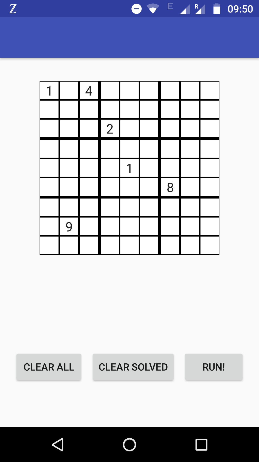
I wrote a sudoku solver in Python as a little toy project, but wanted to make it feel a bit more real so I rewrote it in Javascript so that all the world can solve their sudokus.

If there is a solution, the program will find it. But beware: the method used is not very sophisticated, so if there not a solution, your browser might get upset while it searches through all the incorrect solutions.

See code on Github here.

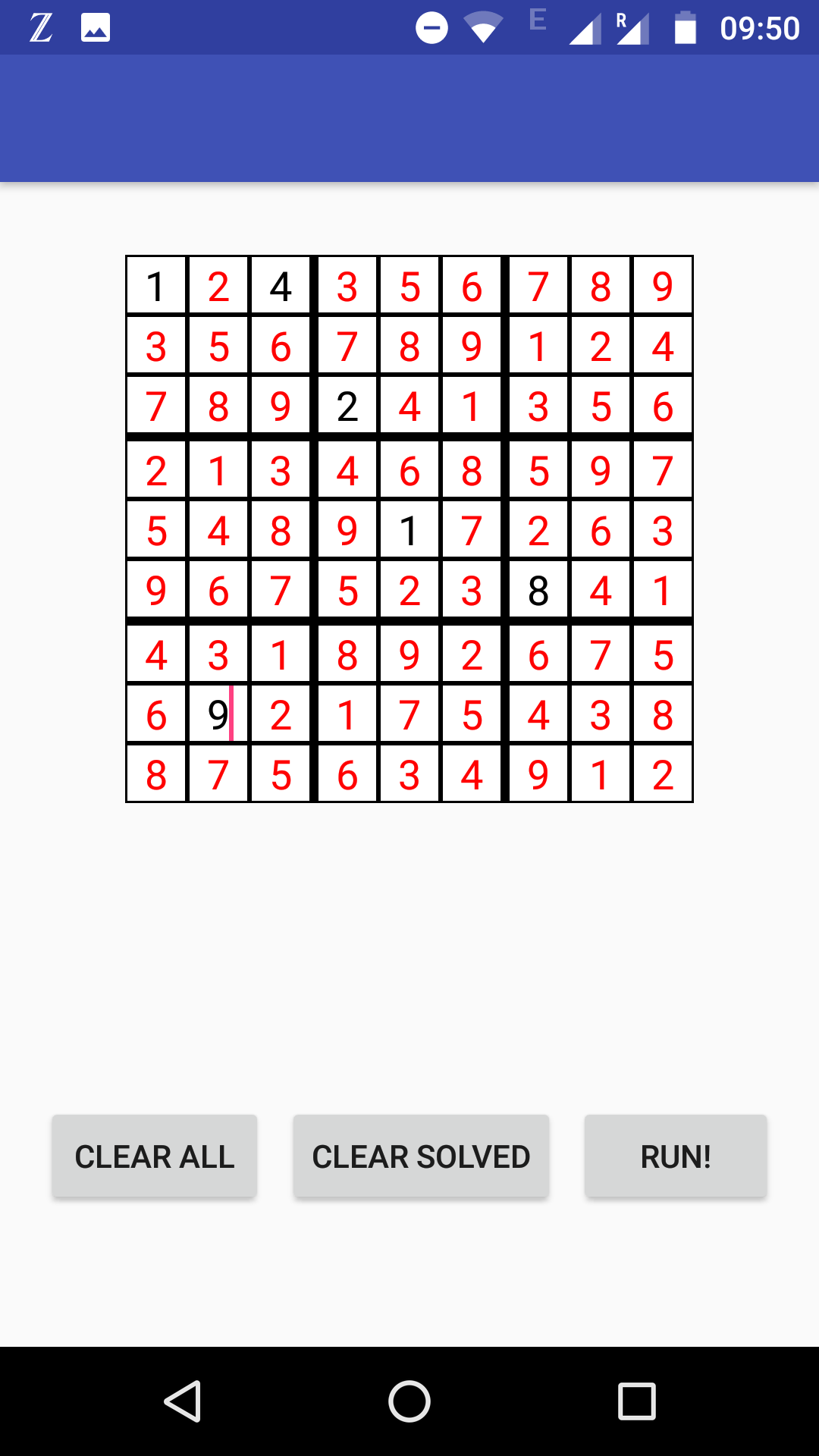
Update: I also made an Android App of this – it was quite a challenge as I’m only very vaguely familiar with Java and had only once before played around with Android once a few years ago. There’s certainly room for improvement here, but I’m pleased to have made something that I can actually interact with on my phone. The code for this is also on the Github repo.

sudoku_android1 sudoku_android2

Interactive Voronoi Partitions using D3

D3 is a powerful Javascript library for in-browser interactive data visualisations. During my masters in Computational Biology, Voronoi Paritions were one of the tools I used to analyse the patterns formed by retinal cells throughout development.

Here is a little demo of Voronoi Partitions I made to learn a bit of d3. Code available on github.

Click and drag a point to move it. Double click a point to delete it.
Double click anywhere else to add a new point.

Neural art

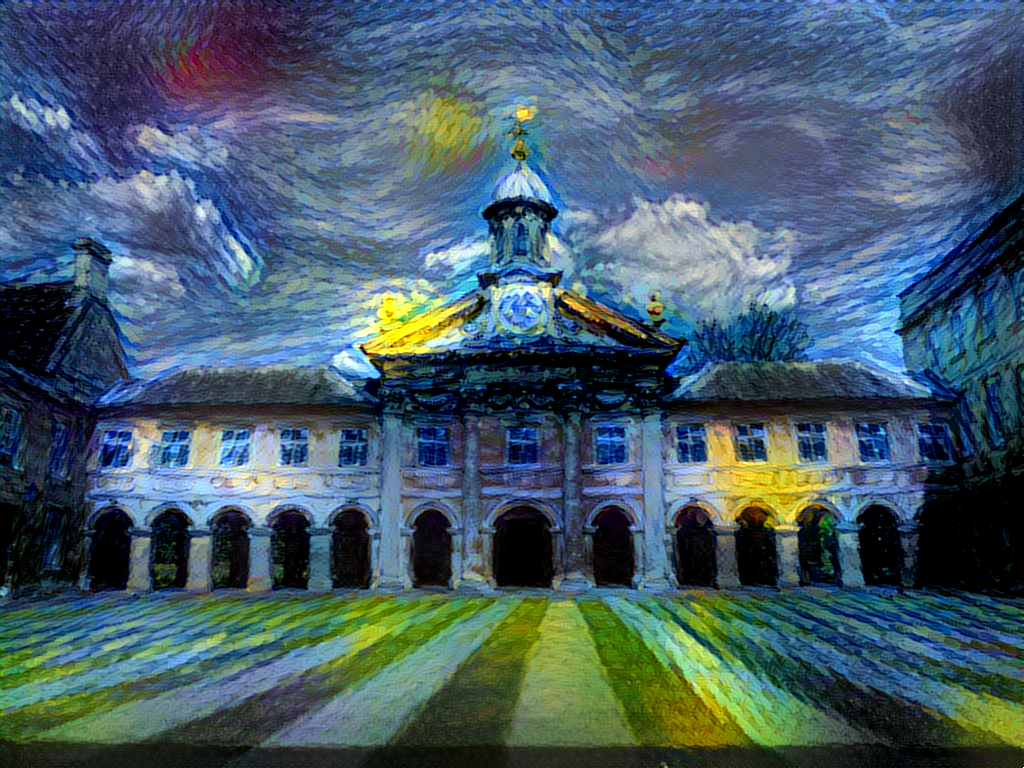
Around the Christmas break I was playing with Leon Gatys et al’s Neural Algorithm of Artistic Style using the open source implementation by Justin Johnson. Here are a few images that I thought were cool!


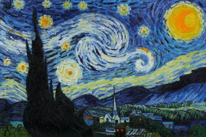
Emmanuel College in the style of The Starry Night

emmanuelstarry


emmanuel-starry-big2


Clare College Bridge and Monet’s Waterlilies

clare_bridgemonet_lilly


clare_bridge_monet_lilly


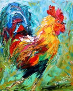
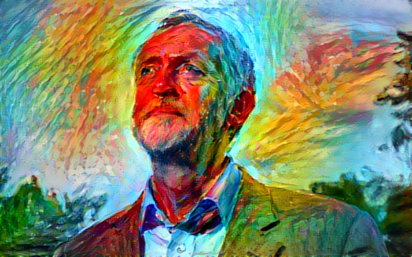
Jeremy Corbyn in the style of an impressionist rooster

chicken


corbyn_chicken


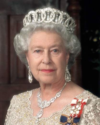
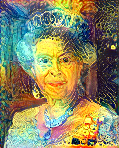
The Queen in the style of some “LSD art”

queenLizzylsd


queen_lsd


The incredible Akhil, also drawn in the style of some “LSD art”


akhil_twinlsd


akhil_twin_lsd_big


This is a video of the above image being generated. When running the programme the makes the blended images, a loop is run for a large number of iterations (~2000 times). The frames of this video show the image above after each multiple of 5 iterations.